How to find acquaintances or contacts through simple data analysis

Learn how simple data mining techniques can help you find people or their contacts. A step-by-step guide for those who want to get the information they need easily and quickly, even if you have no experience in this topic. In the article, you will find step-by-step instructions that will help you easily and quickly get the information you need, even without special knowledge.

Let’s start

Let’s get startedMany researchers, when looking at accounts in social networks, limit themselves to a quick look at the latest posts or bio. However, it is possible to conduct a full analysis of the account, identifying the main themes of the content or filtering out unnecessary material.

This article explains how you can use Google Sheets to filter posts with original content and identify the most common words in an account, without specifying usernames.

The Osint Combine Twitter account (@osintcombine) is used as an example. The process of obtaining such data will be discussed in detail in a separate publication. The described methods are suitable for working with any types of data.

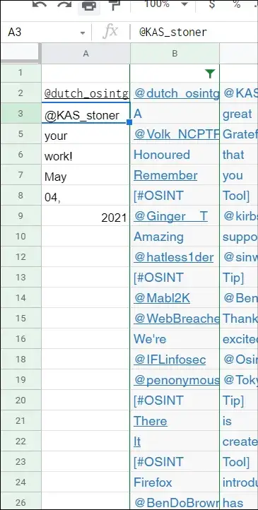
Для початку перейдіть до Google Таблиць ( https://docs.google.com/spreadsheets/u/0/ ) and paste the tweets into the column. in cell B2.

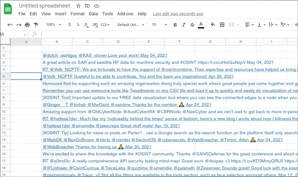
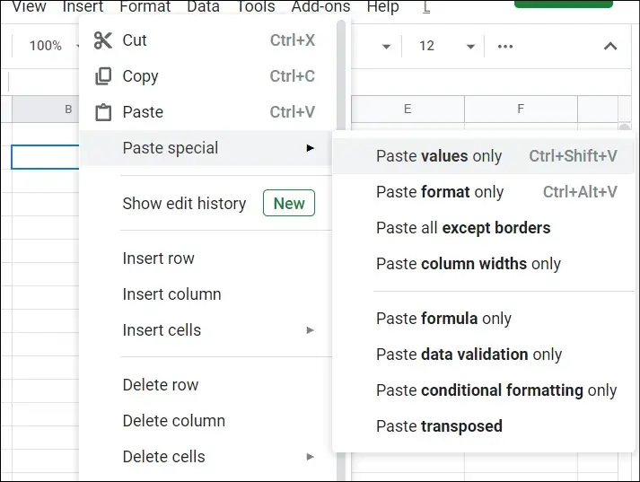
If you want to remove all formatting, instead of pasting into a cell normally, you can right-click on the cell and select Paste Special, then select the Paste Values ​​Only option.

How to filter out irrelevant words

Many irrelevant words such as “the” or “at” can be filtered out by excluding words shorter than a specified minimum number of characters. After that, you can find and delete all words that contain 6 characters or less.

1. Select everything by pressing CTRL and A at the same time.

2. Click Edit and then Find and Replace.

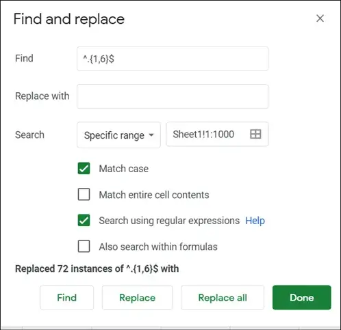
3. In the new box next to Find, type the following: ^.{1,6}$ NOTE: This is a “regex” that applies to all words between 1 and 6 characters long. Change the numbers as you like for your own spreadsheet.

4. Next to ‘replace with’, enter a space.

5. Check the box next to “search by regular expressions” and then click “Replace all”

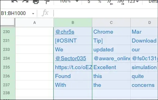
Now the screen looks like this, with lots of gaps.

How to count words

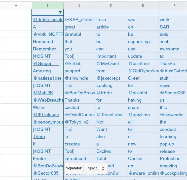
First, select the column of texts, then click Data, Split Text to Columns, and then in the small Splitter window that appears, click the drop-down menu and select Space.

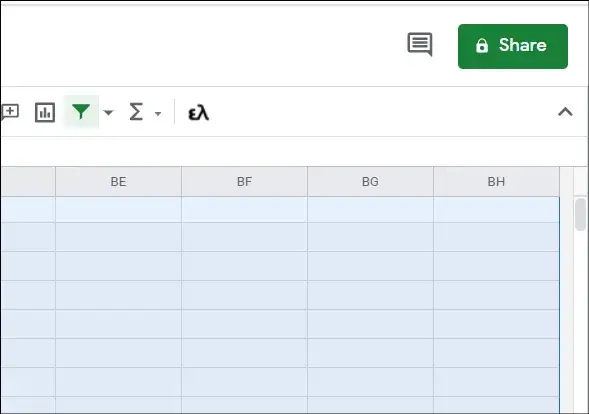
And across all the way to the BH column. Note that the ‘break text into columns’ tool will highlight columns if they have data (so you know you’ve reached the end of the columns when they’re no longer highlighted).

This means that the data covers the range from field B2 in the upper left to BH237 in the lower right. At the next stage, enter the formula =FLATTEN(B2) in field A2 and press Enter. This action combines all data from the selected range into one column.

All individual words will now be displayed in column A. It should be noted that at first column A may appear to contain blank spaces. This is due to the blank cells being included, but scroll down and the rest of the data becomes visible.

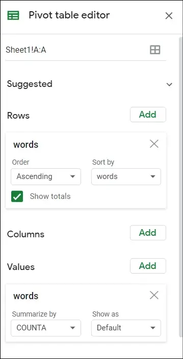
At the next stage, you should enter a title in cell A1, for example “words”. After that, select column A, go to the Data menu, choose Pivot Table, make sure the New Sheet option is selected in the dialog box, and click New.

In the panel on the right next to the Rows section, click Add and select words (or the name entered in cell A1). Next, under the Meaning section, click Add and select words again. By default, Summarize By should be set to COUNTA.

Delete usernames?

At this point, you can choose to remove all usernames from your data. To do this, select column A, select Data, then Filter View, and click Create New Filter View.

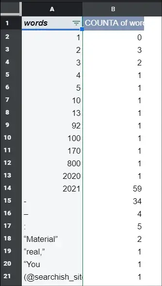
Then click on the upside-down arrow next to the “words” heading in A1 and select sort A-Z. After that, all numbers and unusual characters will be placed at the beginning of the list.

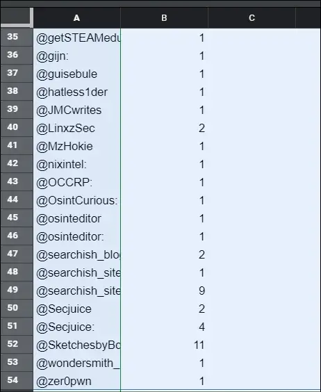
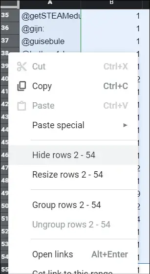
If you scroll down, you can see all the usernames because they start with the @ symbol. To delete these rows, left-click the row number next to the first username, then hold Shift and click the row number next to the last username.

Then right-click anywhere on the row numbers and choose hide all rows.

Alternatively, you can choose to view only usernames by highlighting all other rows without usernames and hiding them.

Easier way to list or delete usernames?

An alternative step.

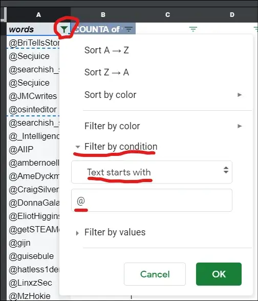
Select column A, go to the Data menu, select Filter View, and then select Create New Filter View. After that, click on the upside-down arrow next to the “words” heading in A1.

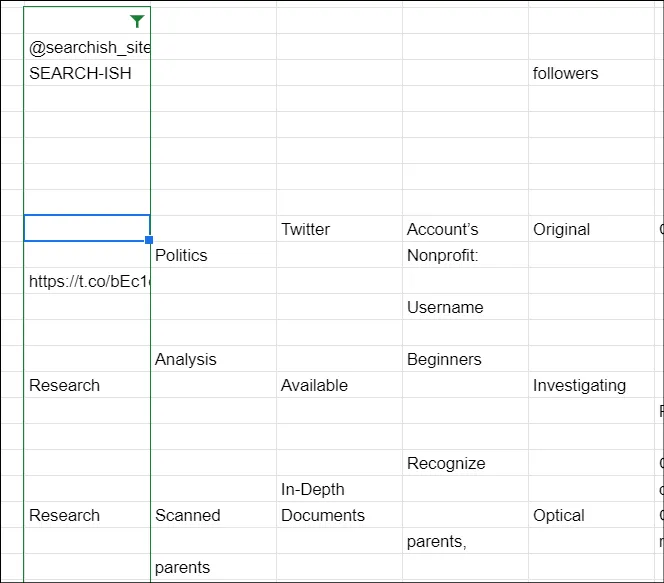
To filter only usernames, select Filter by condition from the drop-down menu, then select Text starts with and enter the @ symbol. This will display all usernames starting with the @ symbol.

You can spot duplicate usernames, such as “@searchish” and “@searchish:” because of characters like commas or colons at the end. To solve this problem, you need to go back to the first step, and after that, go to “Edit”, choose “Find and replace”, then look for the symbol “:” and replace it with a space ” “. Click Replace All.

If the goal is to exclude usernames, after selecting “Filter by condition” you should select “Text does not contain” instead of “Text starts with”.

Explore the most popular usernames?

If the goal is to find the most common usernames, you can do additional research by looking for different accounts or email addresses that use the same usernames. This allows for simultaneous monitoring of multiple sources of information for deeper analysis.

Now whether you have deleted your usernames or not, proceed as follows

You can now exit the filter view by clicking the X in the right corner. You may have to close the PivotTable editor first to see this button.

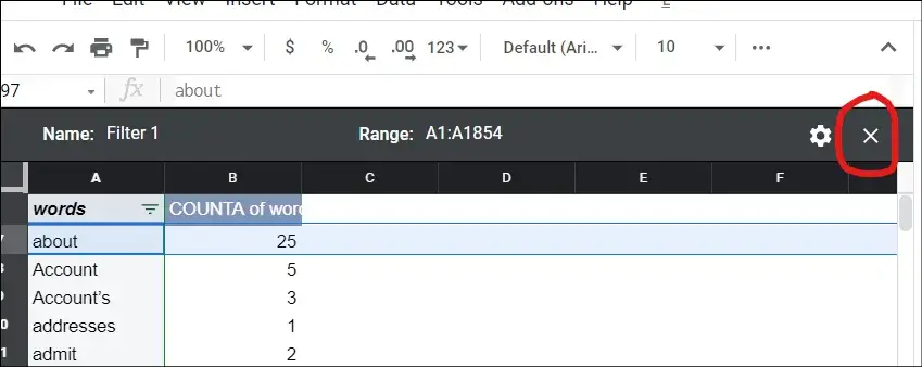
Next, click on the small empty box in the upper left corner above the “1” marker for row 1 to highlight all the data on the sheet.

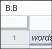
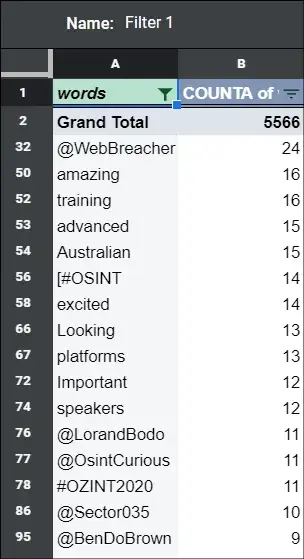
Click Data, Filter View, then Create New Filter View and click the small inverted triangle in column B and select Sort A->A.

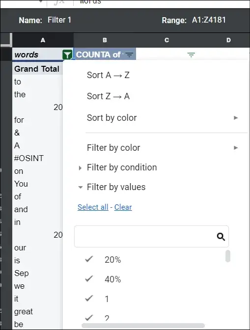
And now we see: